Reinforcement Learning for Autonomous Driving

Part 1: RL background

Maximilian Igl, NVIDIA

Slides: maximilianigl.com/blog

Why RL

• Why RL
• Policy gradients and the critic
• PPO
• GRPO
• RL Landscape
• Data moves

Covariate Shift

• Supervised training only ever sees expert states.
• The model hasn’t learned to recover from it’s own mistakes
• Small mistakes compound over time

Solution. Train the model on in closed loop, i.e. on its own rollouts.

Ross, Gordon, Bagnell. A reduction of imitation learning to no-regret online learning (DAgger), 2011
Karkus, Igl et al. Beyond behavior cloning in autonomous driving: a survey of closed-loop training techniques, preprint

Are there alternatives to RL?

Core problem: Finding the best action in a visited state for which we don’t have data.

RL: Find highest reward action from exploration.

• Expensive and sample-inefficient
• Made affordable by :
  • Generalisation of models across states
  • Pre-training

Using an Oracle: Something supplies optimal action \(a^*(s)\).

Example oracles:

• Human, as in the original DAgger
• A privileged policy, such as a planner that sees the full state
• A policy-improvement operator, such as MCTS on top of the current network in AlphaGo Zero.

Ross, Gordon, Bagnell. A reduction of imitation learning to no-regret online learning (DAgger), 2011
Silver et al. Mastering the game of Go without human knowledge (AlphaGo Zero), 2017

Experimental Evidence

Closed-loop fine-tuning improves performance of strong pre-trained base policy.

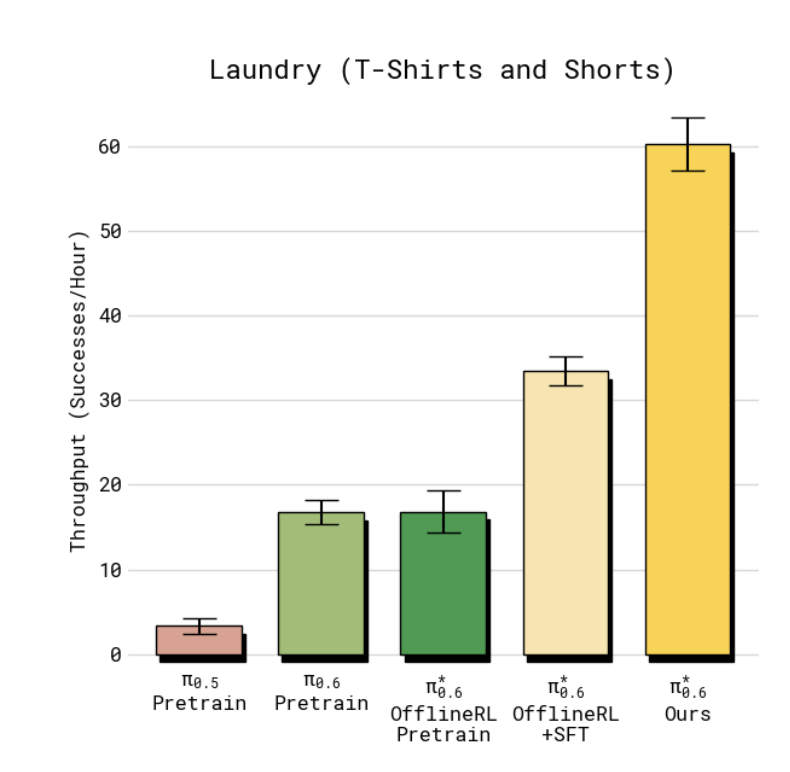
π*0.6, Physical Intelligence, 2025. Laundry folding, successes per hour. RL on the robot’s own deployment experience roughly doubles throughput.

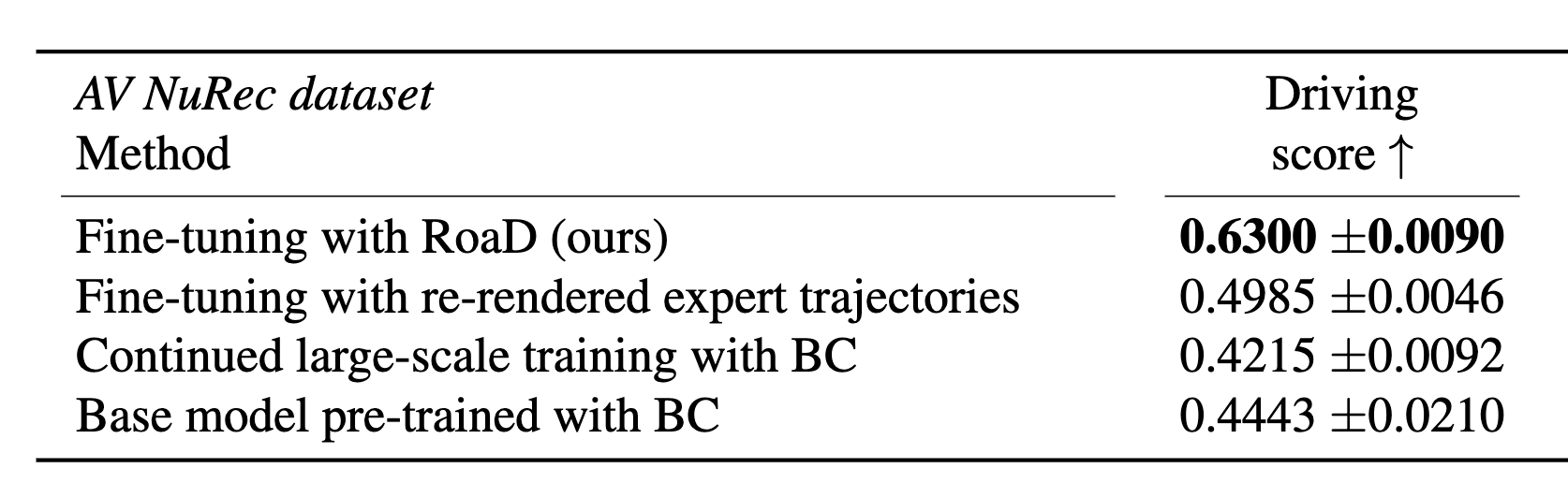
RoaD, Garcia-Cobo et al., 2025. An E2E driving policy fine-tuned on its own closed-loop rollouts.

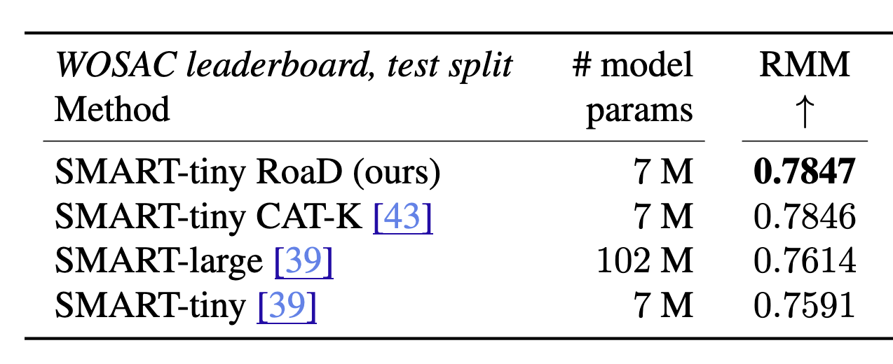
RoaD on WOSAC. Closed-loop fine-tuning (Cat-K) outperforms a 15 times larger pretrained policy.

Garcia-Cobo et al. RoaD: rollouts as demonstrations for closed-loop SFT of driving policies, 2025
Zhang et al. Closed-loop supervised fine-tuning of tokenized traffic models (CAT-K), 2024
Amin et al. π*0.6: a VLA that learns from experience, 2025

RL for Superhuman Performance

AlphaGo, 2016. Human-game training followed by self-play.

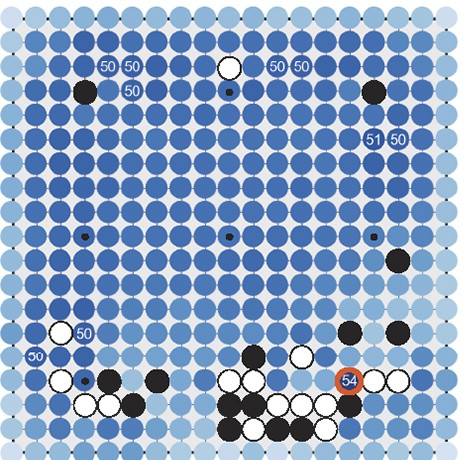
Silver et al., Nature 2016. Fig. 5a. The value network’s estimate for every point on the board.

AlphaZero, 2017. Beating Stockfish with no human games.

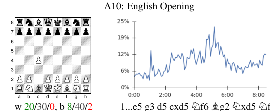
Silver et al., Science 2018. Fig. 2. The English Opening, and how often self-play used it over training. AlphaZero found the human openings by itself, then dropped some.

Fusion, 2022. Plasma shape control in a tokamak, DeepMind and EPFL.

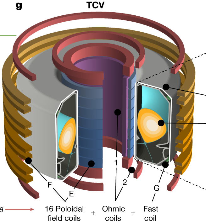
Degrave et al., Nature 2022. Fig. 1g. The TCV tokamak. The policy sets 19 coil voltages from 92 measurements, trained in simulation and run on the real machine.

Simulator + reward + exploration allows the model to find superhuman policies.

Silver et al. Mastering the game of Go with deep neural networks and tree search, 2016
Silver et al. A general RL algorithm that masters chess, shogi, and Go through self-play, 2018
Degrave et al. Magnetic control of tokamak plasmas through deep RL, 2022

RL for LLMs

RLHF. (RL from Human Feedback)

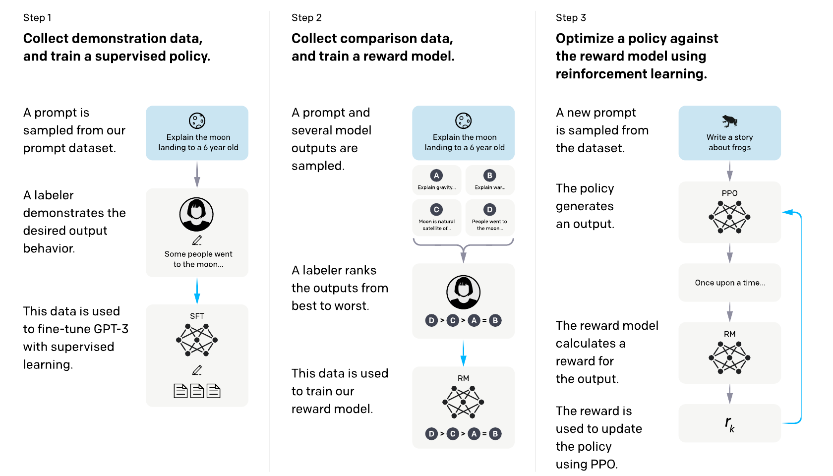
InstructGPT, Ouyang et al. 2022, Fig. 2. Humans rank sampled answers, a reward model learns the ranking, PPO optimises against it with a KL penalty to the supervised model.

RLVR. (RL with Verifiable Rewards)

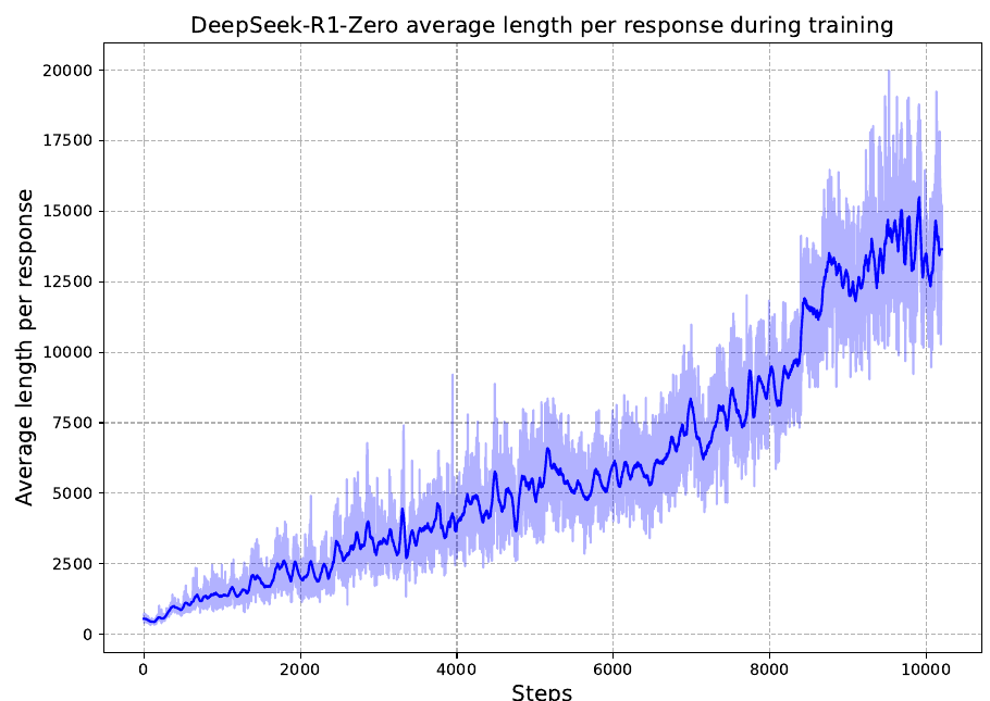
DeepSeek-R1, 2025, Fig. 1b. A checker scores the final answer, nothing else. Trained on correctness alone, the model learns to think longer: response length during RL.

And RL even works for very large models!

Ouyang et al. InstructGPT, 2022
Rafailov et al. DPO, 2023
Lambert et al. Tülu 3 (RLVR), 2024
DeepSeek-AI. DeepSeek-R1, 2025
Gao, Schulman, Hilton. Scaling laws for reward model overoptimization, 2022
Yue et al. Does RL really incentivize reasoning capacity beyond the base model?, 2025

Policy gradients and the critic

• Why RL
• Policy gradients and the critic
• PPO
• GRPO
• RL Landscape
• Data moves

The Markov decision process (MDP)

• State \(s_t \in \mathcal S\), action \(a_t \in \mathcal A\)
• Transition \(s_{t+1} \sim P(\cdot \mid s_t, a_t)\): the environment transition
• Reward \(r_t = r(s_t, a_t)\)
• Policy \(a_t \sim \pi_\theta(\cdot \mid s_t)\)
• Return \(R(\tau) = \sum_{t=0}^{T} \gamma^{t} r_t\), discount \(\gamma \in [0,1)\)
• Objective \(J(\pi_\theta) = \mathbb E_{\tau \sim \pi_\theta}\left[R(\tau)\right]\)
• Value \(V^\pi(s) = \mathbb E\left[\sum_{k\ge 0} \gamma^k r_{t+k} \mid s_t = s\right]\), so \(J(\pi) = \mathbb E_{s_0}\left[V^\pi(s_0)\right]\)
• Action value \(Q^\pi(s,a)\), the same but conditioning on \(a_t = a\)

Two different approaches for RL

Optimizing the policy vs. optimizing the value function.

Policy-based Parametrise \(\pi_\theta\) and ascend \(\nabla_\theta J(\pi_\theta)\).

E.g. REINFORCE, A2C, TRPO, PPO, GRPO.

\[ \nabla_\theta J(\pi_\theta) = \mathbb E_{\tau \sim \pi_\theta}\Big[\sum_t \nabla_\theta \log \pi_\theta(a_t \mid s_t)\, R(\tau)\Big] \]

Value-based. Learn \(Q(s,a)\) from Bellman consistency.

E.g. Q-learning, DQN, and the continuous-action DDPG and SAC.

\[ Q(s,a) \leftarrow r + \gamma \max_{a'} Q(s', a') \]

I will focus on policy-based methods here as they are more widely used in AV for continuous actions.

Five steps from the sampled gradient to PPO

1. The log-derivative trick
2. Variance reduction with the advantage \(A^\pi = Q^\pi - V^\pi\)
3. Learning the critic \(V_\phi(s) \approx V^\pi(s)\)
4. Generalised advantage estimation \(\hat A_t = \sum_{l} (\gamma\lambda)^l\, \delta_{t+l}\)
5. Batch reuse and clipping

REINFORCE: the log-derivative trick

The log-derivative trick estimates the policy gradient without backpropagating through the environment.

\[ p_\theta(\tau) = \rho(s_0)\, \prod_{t=0}^{T} \pi_\theta(a_t \mid s_t)\, {\color{#b5452f} P(s_{t+1} \mid s_t, a_t)} \]

The environment \(P\) is unknown and not differentiable, so \(\nabla_\theta p_\theta(\tau)\) cannot be taken directly.

\[ \nabla_\theta J = \nabla_\theta \int p_\theta(\tau)\, R(\tau)\, d\tau \]

\[ = \int {\color{#2f6f3e} p_\theta(\tau)\, \nabla_\theta \log p_\theta(\tau)}\, R(\tau)\, d\tau \]

\(\nabla p = p\, \nabla \log p\). Log-derivative trick.

\[ = {\color{#2f6f3e} \mathbb E_{\tau \sim p_\theta}}\left[\nabla_\theta \log p_\theta(\tau)\, R(\tau)\right] \]

Monte Carlo estimate from rollouts is unbiased!

\[ = \mathbb E_{\tau \sim p_\theta}\left[{\color{#2f6f3e} \sum_{t=0}^{T} \nabla_\theta \log \pi_\theta(a_t \mid s_t)}\; R(\tau)\right] \]

Only \(\log \pi_\theta(a_t \mid s_t)\) depends on \(\theta\), the rest drops: \(\log p_\theta(\tau) = \log \rho(s_0) + \sum_t \log \pi_\theta + \sum_t \log P\).

Variance reduction using advantage estimation.

The biggest problem in RL is noise / gradient variance.

\[ \nabla_\theta J = \mathbb E\left[\sum_t \nabla_\theta \log \pi_\theta(a_t \mid s_t)\; R(\tau)\right] \]

\[ = \mathbb E\left[\sum_t {\color{#2f6f3e} \gamma^t}\, \nabla_\theta \log \pi_\theta(a_t \mid s_t)\; {\color{#2f6f3e} \hat R_t}\right], \qquad {\color{#2f6f3e} \hat R_t = \sum_{t' \ge t} \gamma^{t'-t} r_{t'}} \]

Reward-to-go is enough. The \(\gamma^t\) discounts from the episode start.

\[ = \mathbb E\left[\sum_t \gamma^t\, \nabla_\theta \log \pi_\theta(a_t \mid s_t)\; \big(\hat R_t\, {\color{#2f6f3e} - b(s_t)}\big)\right] \]

Any baseline \(b(s_t)\) is free, as long as it does not depend on \(a_t\):
\(\mathbb E_{a \sim \pi_\theta}\!\left[\nabla_\theta \log \pi_\theta(a \mid s)\, b(s)\right] = b(s)\, \nabla_\theta \textstyle\sum_a \pi_\theta(a \mid s) = 0\).

\[ = \mathbb E\left[\sum_t \gamma^t\, \nabla_\theta \log \pi_\theta(a_t \mid s_t)\; {\color{#2f6f3e} \underbrace{\big(\hat R_t - V^\pi(s_t)\big)}_{\hat A(s_t,\, a_t)}}\right] \]

Advantage \(\hat A(s_t, a_t)\): how much better than average was \(a_t\) in \(s_t\)?

\[ \hat A(s_t, a_t) \approx {\color{#2f6f3e} r_t + \gamma\, V^\pi(s_{t+1})} - V^\pi(s_t) \]

Another way to estimate \(\hat A(s_t, a_t)\) from one step: less variance, but more biased.

Temporal Difference learning for the critic \(V\)

Two ways to fit the critic: regress on Monte Carlo returns, or bootstrap with temporal-difference targets.

\[ V^\pi(s_t) = \mathbb E\left[r_t + \gamma r_{t+1} + \gamma^2 r_{t+2} + \dots\right] = \mathbb E\big[\hat R_t\big] \]

\[ {\color{#2f6f3e} \mathcal L_{\mathrm{MC}}(\phi)} = \mathbb E\left[\big({\color{#2f6f3e} V_\phi(s_t)} - \hat R_t\big)^2\right] \]

1. Monte Carlo: regress on the reward-to-go of whole rollouts. Unbiased, but high variance.

\[ V^\pi(s_t) = \mathbb E\Big[r_t + \gamma \underbrace{\big(r_{t+1} + \gamma r_{t+2} + \dots\big)}_{\color{#2f6f3e} V^\pi(s_{t+1})}\Big] = \mathbb E\left[r_t + \gamma\, {\color{#2f6f3e} V^\pi(s_{t+1})}\right] \]

2. Temporal difference: pull out the first reward, the rest is \(V^\pi(s_{t+1})\).

\[ {\color{#2f6f3e} \mathcal L(\phi)} = \mathbb E\left[\big({\color{#2f6f3e} V_\phi(s_t)} - r_t - \gamma\, {\color{#2f6f3e} V_{\bar\phi}(s_{t+1})}\big)^2\right] \]

TD learning: one sampled transition, \(V_\phi\) in place of \(V^\pi\), no gradient through the target (\(\bar\phi\)). Low variance, but biased while \(V_\phi\) is wrong.

Temporal Difference learning for the critic \(V\)

Visual example of how \(V^\pi\) is learned.

\[ V^\pi(s) \leftarrow \sum_{a} \pi(a \mid s)\, \sum_{s'} P(s' \mid s, a)\,\big[r + \gamma\, V^\pi(s')\big] \]

GAE interpolates between one-step TD and Monte Carlo estimates

Two estimates of the same advantage, from the variance-reduction slide:

• Monte Carlo, \(\hat R_t - V_\phi(s_t)\): unbiased, but the variance of a long sum of rewards.
• One-step, \(r_t + \gamma V_\phi(s_{t+1}) - V_\phi(s_t)\): low variance, but the critic’s bias.

GAE interpolates between them.

\[ \delta_t = r_t + \gamma V_\phi(s_{t+1}) - V_\phi(s_t) \]

The one-step estimate, named: the TD error.

\[ \hat A_t^{\mathrm{GAE}(\gamma,\lambda)} = \sum_{l \ge 0} {\color{#2f6f3e} (\gamma \lambda)^l}\, \delta_{t+l} \]

An exponentially weighted sum of them.

\[ \hat A_t = -V_\phi(s_t) + {\color{#2f6f3e} r_t} + \gamma\lambda\, {\color{#2f6f3e} r_{t+1}} + \gamma^2\lambda^2\, {\color{#2f6f3e} r_{t+2}} + \cdots \]

\[ \phantom{\hat A_t = -V_\phi(s_t)}\; + \gamma(1-\lambda)\, {\color{#2f6f3e} V_\phi(s_{t+1})} + \gamma^2 \lambda (1-\lambda)\, {\color{#2f6f3e} V_\phi(s_{t+2})} + \cdots \]

Written out the full interpolation between rewards and critics.

\[ \lambda = 0:\ \hat A_t = \delta_t \qquad\qquad \lambda = 1:\ \hat A_t = \hat R_t - V_\phi(s_t) \]

The two ends: the one-step estimate, and Monte Carlo minus the baseline.

PPO uses this estimate with \(\lambda \approx 0.95\): nearly Monte Carlo, with the critic damping the variance.

Schulman et al. High-dimensional continuous control using generalized advantage estimation, 2015

PPO

• Why RL
• Policy gradients and the critic
• PPO
• GRPO
• RL Landscape
• Data moves

The algorithm so far

Roll out, estimate advantages, one gradient step

Algorithm 1 Actor-critic policy gradient, as assembled so far

for iteration \(k = 1, 2, \dots\) do

1. \(\mathcal D = \{(s_t, a_t, r_t, s_{t+1})\},\ |\mathcal D| = NT\) Run \(\pi_\theta\) in \(N\) environments for \(T\) steps each.
2. \(\hat A_t = \sum_{l \ge 0} (\gamma\lambda)^l\, \delta_{t+l}\) GAE on the TD errors \(\delta_t = r_t + \gamma V_\phi(s_{t+1}) - V_\phi(s_t)\).
3. \(\theta \leftarrow \theta + \alpha \sum_{\mathcal D} \nabla_\theta \log \pi_\theta(a_t \mid s_t)\, \hat A_t\) One gradient step on the policy.
4. \(\phi \leftarrow \phi - \beta\, \nabla_\phi \sum_{\mathcal D} \big(V_\phi(s_t) - \hat V_t\big)^2\) One critic step, target \(\hat V_t = \hat A_t + V_\phi(s_t)\).
5. Discard the batch.

end for

The problem: Rollouts are expensive and each batch buys only one gradient step.

PPO reuses each batch by correcting for the policy that collected it

PPO’s ratio is the importance weight that lets \(\pi_{\mathrm{old}}\)’s samples estimate \(\pi_\theta\)’s gradient.

\[ \nabla_\theta J = \mathbb E_{a_t \sim \pi_\theta}\left[\nabla_\theta \log \pi_\theta(a_t \mid s_t)\, \hat A_t\right] \]

\[ = \mathbb E_{{\color{#2f6f3e} a_t \sim \pi_{\mathrm{old}}}}\left[{\color{#2f6f3e} \frac{\pi_\theta(a_t \mid s_t)}{\pi_{\mathrm{old}}(a_t \mid s_t)}}\, \nabla_\theta \log \pi_\theta(a_t \mid s_t)\, \hat A_t\right] \]

Importance sampling, \(\mathbb E_{p}[f] = \mathbb E_{q}\big[\tfrac{p}{q}\, f\big]\).

\[ = \mathbb E_{a_t \sim \pi_{\mathrm{old}}}\left[\frac{{\color{#2f6f3e} \nabla_\theta\, \pi_\theta(a_t \mid s_t)}}{\pi_{\mathrm{old}}(a_t \mid s_t)}\, \hat A_t\right] \]

The log-derivative trick in reverse: \(\pi_\theta\, \nabla_\theta \log \pi_\theta = \nabla_\theta \pi_\theta\).

\[ = {\color{#2f6f3e} \nabla_\theta}\, \mathbb E_{a_t \sim \pi_{\mathrm{old}}}\left[{\color{#2f6f3e} r_t(\theta)}\, \hat A_t\right], \qquad r_t(\theta) = \frac{\pi_\theta(a_t \mid s_t)}{\pi_{\mathrm{old}}(a_t \mid s_t)} \]

\(\pi_{\mathrm{old}}\) and \(\hat A_t\) do not depend on \(\theta\), so the gradient moves outside.

Off-policy problems:

• The weight only adjusts the actions, not the states.
• The advantages were estimated for \(\pi_{\mathrm{old}}\), not \(\pi_\theta\).
• The importance ratio can explode.

Schulman et al. Proximal policy optimization algorithms, 2017

Clipping removes the incentive to push \(r\) past \(1 \pm \epsilon\)

The PPO trick: Clipping removes the gradient only when we moved too far into beneficial directions.

\[ L^{\mathrm{CLIP}}(\theta) = \mathbb E_t\left[\min\Big(r_t(\theta)\hat A_t,\ \operatorname{clip}\big(r_t(\theta), 1-\epsilon, 1+\epsilon\big)\hat A_t\Big)\right] \]

\(\hat{A} > 0\): Positive advantage, we want to increase the probability of this action!

\(r > 1\): Probability of this action is increased!

\(\hat A > 0,\ r > 1+\epsilon\). Flat: no gradient, pushed up enough.

\(\hat A > 0\), otherwise. Pushes \(r\) up, also back from below \(1-\epsilon\).

\(\hat A < 0,\ r < 1-\epsilon\). Flat: no gradient, pushed down enough.

\(\hat A < 0\), otherwise. Pushes \(r\) down, also back from above \(1+\epsilon\).

Clipping removes the incentive to push too hard on improving the advantage on data that is too off-policy while never removing gradients from data where we unlearned something.

The full PPO algorithm

Alternate rollouts with multiple gradient updates on minibatches.

Algorithm 2 PPO: Algorithm 1 with the batch reused, \(K \cdot NT / M\) gradient steps per rollout instead of one

for iteration \(k = 1, 2, \dots\) do

1. \(\mathcal D = \{(s_t, a_t, r_t, s_{t+1})\},\ |\mathcal D| = NT\) Run \(\pi_{{\color{#2f6f3e} \theta_{\mathrm{old}}}}\) in \(N\) environments for \(T\) steps each.
2. \(\hat A_t = \sum_{l \ge 0} (\gamma\lambda)^l\, \delta_{t+l}\) GAE on the TD errors, once, under \(\pi_{\theta_{\mathrm{old}}}\).
3. \({\color{#2f6f3e} \mathcal D = B_1 \cup \dots \cup B_{NT/M}}\) for \(K\) epochs, for each minibatch \(B\) of size \(M\) do
4. \(\theta \leftarrow \theta + \alpha\, \nabla_\theta \textstyle\sum_{B} {\color{#2f6f3e} L^{\mathrm{CLIP}}_t(\theta)}\) One gradient step on the policy, on the clipped ratio.
5. \(\phi \leftarrow \phi - \beta\, \nabla_\phi \textstyle\sum_{B} \big(V_\phi(s_t) - \hat V_t\big)^2\) One critic step, target \(\hat V_t = \hat A_t + V_\phi(s_t)\).
6. \({\color{#2f6f3e} \theta_{\mathrm{old}} \leftarrow \theta}\) Discard the batch.

end for

Schulman et al. Proximal policy optimization algorithms, 2017

GRPO

• Why RL
• Policy gradients and the critic
• PPO
• GRPO
• RL Landscape
• Data moves

GRPO drops the critic and uses the group as the baseline

Sample \(G\) whole trajectories \(\tau_1, \ldots, \tau_G\) from the same prompt or state, one reward each.

\[ \hat A_i = \frac{R_i - \operatorname{mean}(R_{1:G})}{{\color{#2f6f3e} \operatorname{std}(R_{1:G})}} \]

The group mean is the baseline: no critic, and one advantage for the whole trajectory.

\[ L = \mathbb E\left[\min\big(r_i \hat A_i,\ \operatorname{clip}(r_i)\hat A_i\big)\right] - {\color{#2f6f3e} \beta\, D_{\mathrm{KL}}\big(\pi_\theta \,\|\, \pi_{\mathrm{ref}}\big)} \]

The rest is PPO’s clipped objective, plus a KL regularization to the pretrained model.

Later variants change the green parts:

• Dr. GRPO drops the std, which over-weights very easy and very hard prompts.
• DAPO drops the KL term, raises the upper clip bound, and resamples groups with all-equal rewards.
• Lite PPO keeps the group mean but takes the std over the whole batch.

Shao et al. DeepSeekMath (GRPO), 2024
Liu et al. Understanding R1-Zero-like training (Dr. GRPO), 2025
Yu et al. DAPO, 2025
Liu et al. Tricks or traps? A deep dive into RL for LLM reasoning (Lite PPO), 2025

The broader RL landscape

• Why RL
• Policy gradients and the critic
• PPO
• GRPO
• RL Landscape
• Data moves

Exploration decides what even can be learned

A simple example for the exploration / exploitation tradeoff.

Local optimum. A greedy learner starts going only left.

Collapse. Without an entropy bonus the optimum of \(J(\theta)\) is a deterministic policy.

Exploration bonus Entropy regularization, curiosity, and curricula keep the policy exploring, but exploration is mostly undirected.

Strehl, Littman. An analysis of model-based interval estimation for Markov decision processes (RiverSwim), 2008

Offline RL overestimates unobserved actions.

Offline RL: Fixed data, never roll out the policy. Here we examine the failure mode of value learning.

\[ \mathcal L(\phi) = \mathbb E\Big[\big(Q_\phi(s_t, a_t) - r_t - \gamma \max_{a'} Q_{\bar\phi}(s_{t+1}, a')\big)^2\Big] \]

Problem: The \(\max_{a'}Q\) operator is biased towards the value that is most overestimated due to random noise.

Propagation: An inflated value is the target of its neighbours.

No feedback. Online RL would take the overrated action, see its real return, and correct the value. Offline RL never gets to try it.

Inference: \(\arg\max_a Q\) from \(s_0\) loops and never reaches the goal.

Solution: CQL penalizes high values for actions poorly supported by the dataset.

Transfer to PPO: A conservative critic may need recalibration: pessimistic values can bias bootstrapped advantages.

Kumar et al. Conservative Q-learning for offline RL, 2020

Model-based RL learns the transition function and rolls out inside it

Payoff: sample efficiency. Danger: the policy exploits errors in \(\hat P\).

Example: DreamerV3 (Hafner et al., Nature 2025) does this successfully in a learned latent space.

Hafner et al. Dream to control: learning behaviors by latent imagination (Dreamer), 2020
Hafner et al. Mastering diverse domains through world models (DreamerV3), 2023, in Nature 2025

POMDP: When the state is not observed, the policy needs memory

Driving is a POMDP: A camera does not see intent, occluded agents, or the road friction.

\[ P(s_{t+1} \mid s_t, a_t) = P(s_{t+1} \mid s_0, a_0, \dots, s_t, a_t) \]

Markov. \(s_t\) is a sufficient statistic of the history.

\[ o_t \sim O(\cdot \mid s_t), \qquad P(o_{t+1} \mid o_t, a_t) \ne P(o_{t+1} \mid o_{\le t}, a_{\le t}) \]

POMDP. The policy sees \(o_t\), not \(s_t\). Observations are not Markov!

\[ b_t(s) = P(s_t = s \mid o_{\le t}, a_{<t}) \]

Belief. The posterior over \(s_t\) is Markov again, so a policy on \(b_t\) or on the full history is optimal.

RL: The data moves with the policy

• Why RL
• Policy gradients and the critic
• PPO
• GRPO
• RL Landscape
• Data moves

The moving data distribution is the biggest advantage and disadvantage of RL

Why it helps: The policy trains on states it will actually see

Training on visited states reduces the mismatch and can teach recovery. New strategies can be found and superhuman performance is possible.

Why it is unstable: A bad update changes the data, which makes the next update worse.

Policy collapse can become a feedback loop. Baselines reduce gradient noise; clipping discourages large updates; reference KL and imitation help retain pretrained behaviour.